Understandable Statistics: Concepts and Methods
12th Edition
ISBN: 9781337119917
Author: Charles Henry Brase, Corrinne Pellillo Brase
Publisher: Cengage Learning
expand_more
expand_more
format_list_bulleted
Concept explainers
Videos
Textbook Question
Chapter 9, Problem 9CURP
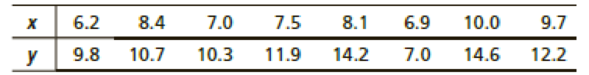
Linear Regression: Blood Glucose Let x be a random variable that represents blood glucose level after a 12-hour fast. Let y be a random variable representing blood glucose level 1 hour after drinking sugar water (after the 12-hour fast). Units are in milligrams per 10 milliliters (mg/10 ml). A random sample of eight adults gave the following information (Reference: American Journal of Clinical Nutrition, Vol. 19, pp. 345–351).
Σx = 63.8; Σx2 = 521.56; Σy = 90.7; Σy2 = 1070.87; Σxy = 739.65
- (a) Draw a
scatter diagram for the data. - (b) Find the equation of the least-squares line and graph it on the scatter diagram.
- (c) Find the sample
correlation coefficient r and the sample coefficient of determination r2. Explain the meaning of r2 in the context of the application. - (d) If x = 9.0, use the least-squares line to predict y. Find an 80% confidence interval for your prediction.
- (e) Use level of significance 1% and test the claim that the population correlation coefficient ρ is not zero. Interpret the results.
- (f) Find an 85% confidence interval for the slope β of the population-based least-squares line. Explain its meaning in the context of the application.
Expert Solution & Answer
Want to see the full answer?
Check out a sample textbook solution
Students have asked these similar questions
3. Regression analysis breaks scores on the DV into... (explain and give equations)
10)
A regression was run to determine if there is a relationship between hours of TV watched per day (x) and number of situps a person can do (y).The results of the regression were:y=ax+b a=-0.767 b=31.009 r2=0.609961 r=-0.781 Use this to predict the number of situps a person who watches 7.5 hours of TV can do (to one decimal place)
The graph below represents a regression line predicting Y from X. This graph shows the error of prediction for each of the actual Y values. Use this information to compute the standard error of the estimate in this sample.
Chapter 9 Solutions
Understandable Statistics: Concepts and Methods
Ch. 9.1 - Statistical Literacy When drawing a scatter...Ch. 9.1 - Prob. 2PCh. 9.1 - Prob. 3PCh. 9.1 - Prob. 4PCh. 9.1 - Prob. 5PCh. 9.1 - Prob. 6PCh. 9.1 - Prob. 7PCh. 9.1 - Prob. 8PCh. 9.1 - Prob. 9PCh. 9.1 - Critical Thinking: Lurking Variables Over the past...
Ch. 9.1 - Prob. 11PCh. 9.1 - Prob. 12PCh. 9.1 - Prob. 13PCh. 9.1 - Health Insurance: Administrative Cost The...Ch. 9.1 - Prob. 15PCh. 9.1 - Geology: Earthquakes Is the magnitude of an...Ch. 9.1 - Prob. 17PCh. 9.1 - Prob. 18PCh. 9.1 - Prob. 19PCh. 9.1 - Prob. 20PCh. 9.1 - Prob. 21PCh. 9.1 - Prob. 22PCh. 9.1 - Prob. 23PCh. 9.1 - Prob. 24PCh. 9.2 - Statistical Literacy In the least-squares line...Ch. 9.2 - Prob. 2PCh. 9.2 - Critical Thinking When we use a least-squares line...Ch. 9.2 - Prob. 4PCh. 9.2 - Prob. 5PCh. 9.2 - Critical Thinking: Interpreting Computer Printouts...Ch. 9.2 - Prob. 7PCh. 9.2 - For Problems 718, please do the following. (a)...Ch. 9.2 - Prob. 9PCh. 9.2 - For Problems 718, please do the following. (a)...Ch. 9.2 - Prob. 11PCh. 9.2 - Prob. 12PCh. 9.2 - For Problems 718, please do the following. (a)...Ch. 9.2 - Prob. 14PCh. 9.2 - Prob. 15PCh. 9.2 - For Problems 718, please do the following. (a)...Ch. 9.2 - Prob. 17PCh. 9.2 - Prob. 18PCh. 9.2 - Prob. 19PCh. 9.2 - Residual Plot: Miles per Gallon Consider the data...Ch. 9.2 - Prob. 21PCh. 9.2 - Prob. 22PCh. 9.2 - Prob. 23PCh. 9.2 - Prob. 24PCh. 9.2 - Prob. 25PCh. 9.3 - Prob. 1PCh. 9.3 - Prob. 2PCh. 9.3 - Prob. 3PCh. 9.3 - Prob. 4PCh. 9.3 - Prob. 5PCh. 9.3 - Prob. 6PCh. 9.3 - Prob. 7PCh. 9.3 - In Problems 712, parts (a) and (b) relate to...Ch. 9.3 - Prob. 9PCh. 9.3 - Prob. 10PCh. 9.3 - In Problems 712, parts (a) and (b) relate to...Ch. 9.3 - Prob. 12PCh. 9.3 - Prob. 13PCh. 9.3 - Prob. 14PCh. 9.3 - Prob. 15PCh. 9.3 - Expand Your Knowledge: Time Series and Serial...Ch. 9.3 - Prob. 17PCh. 9.4 - Statistical Literacy Given the linear regression...Ch. 9.4 - Prob. 2PCh. 9.4 - For Problems 3-6, use appropriate multiple...Ch. 9.4 - For Problems 3-6, use appropriate multiple...Ch. 9.4 - Prob. 5PCh. 9.4 - Prob. 6PCh. 9 - Prob. 1CRPCh. 9 - Prob. 2CRPCh. 9 - Prob. 3CRPCh. 9 - Prob. 4CRPCh. 9 - Prob. 5CRPCh. 9 - Prob. 6CRPCh. 9 - Prob. 7CRPCh. 9 - Prob. 8CRPCh. 9 - Prob. 9CRPCh. 9 - Prob. 10CRPCh. 9 - Prob. 1DHCh. 9 - Prob. 1LCCh. 9 - Prob. 1UTCh. 9 - Prob. 2UTCh. 9 - Prob. 3UTCh. 9 - Prob. 4UTCh. 9 - Prob. 5UTCh. 9 - Prob. 6UTCh. 9 - Prob. 7UTCh. 9 - In Problems 16, please use the following steps (i)...Ch. 9 - Prob. 2CURPCh. 9 - Prob. 3CURPCh. 9 - Prob. 4CURPCh. 9 - Prob. 5CURPCh. 9 - Prob. 6CURPCh. 9 - Prob. 8CURPCh. 9 - Linear Regression: Blood Glucose Let x be a random...
Knowledge Booster


Learn more about
Need a deep-dive on the concept behind this application? Look no further. Learn more about this topic, statistics and related others by exploring similar questions and additional content below.Similar questions
- Respiratory Rate Researchers have found that the 95 th percentile the value at which 95% of the data are at or below for respiratory rates in breath per minute during the first 3 years of infancy are given by y=101.82411-0.0125995x+0.00013401x2 for awake infants and y=101.72858-0.0139928x+0.00017646x2 for sleeping infants, where x is the age in months. Source: Pediatrics. a. What is the domain for each function? b. For each respiratory rate, is the rate decreasing or increasing over the first 3 years of life? Hint: Is the graph of the quadratic in the exponent opening upward or downward? Where is the vertex? c. Verify your answer to part b using a graphing calculator. d. For a 1- year-old infant in the 95 th percentile, how much higher is the walking respiratory rate then the sleeping respiratory rate? e. f.arrow_forwardQuestion 3. a) A Biologist is comparing intervals (m seconds) between the matting calls of a certain species of tree frog and the surrounding temperature (t degree Celsius). The following results were obtained: t 8 13 14 15 15 20 25 30 6.5 4.5 4 3 2 1 1. Fit the regression line in the form m = a + bt. 2. Interpret your estimates. 3. Use your regression line interval between matting calls when the surrounding temperature is 10 degrees. (6 marks) estimate the timearrow_forwardQ1) Interpret the following regression line y = 10.50 – 0.18xarrow_forward
- A random sample of 150 individuals (males and females) was surveyed, and the individuals were asked to indicate their year incomes. The results of the survey are shown below. Income Category Category 1: $20,000 up to $40,000 Category 2: $40,000 up to $60,000 Category 3: $60,000 up to $80,000 Edit Format Table Test at a = .05 to determine if the yearly income is independent of the gender. (CSLO 1,6,7) 12pt Male 10 35 15 V Paragraph BI U A Female 30 15 45 > 2 T² :arrow_forwardA prospective cohort study is run to estimate the incidence of stroke in persons 55 years of age and older. All participants are free of stroke at study start. Each participant is followed for a maximum of 5 years. The data are summarized in Table 3–14. Number of Strokes Number of Stroke-Free Person-Years Men (n = 125) 9 478 Women (n = 200) 21 97 What is the annual incidence rate of stroke in men? What is the annual incidence rate of stroke in women? What is the annual incidence rate of stroke (men and women combined)?arrow_forwardFifty male subjects drank a measured amount x (in ounces) of a medication and the concentration y (in percent) in their blood of the active ingredient was measured 30 minutes later. The sample data are summarized by the following information: n = 50 Ex = 112.5 Ex? = 356.25 %3D Ey = 4.83 Ey = 0.667 Exy = 15.255 0 < x < 4.5 Or= 0.875 Or= 0.709 Or= -0.846 Or=0.460 Or= 0.965arrow_forward
- A random sample of 42 earthquakes that have occurred between January 2015 and September 2017 was selected and for each earthquake the magnitude of the earthquake and the number of people killed was recorded. The data appear in the scatterplot below. 400 350 300 250 200 150 100 50 0 3 -50 4 5 6 7 8 9 10 -100 -150 Magnitude of Earthquake 8 Consider the scatterplot above question 2. Use this scatterplot to describe completely the relationship between the magnitude of the earthquake and the number of people killed. Positive and linear Negative, moderate, linear O Negative, strong, linear Positive, moderate, linear Number of People Killed ---arrow_forwardWe analyze a data set with Y = stopping distance of a car and X = speed of the car when the brakes were applied, %3D and after running the data in STATISTICA, we obtain the following results. Std.Err. of b Std.Err. of b* t(61) p-value b* N=63 Intercept Speed -20.2734 3.1366 -6.26038 20.67978 0.000000 0.000000 3.238368 0.935504 0.045238 0.151674 Sums of df Mean p-value Squares Squares 59540.15 Effect 59540.15 427.6534 0.000000 Regress. Residual 1 8492.74 61 139.23 Total 68032.89 Speed X StopDist Y Speed squared StopDist squared Speed StopDist 65853 Total 1195 2471 28719 164951 One of the observations is (X = 39, Y = 138). The value of the internal studentized residual is . (final answer to 2 decimal places e.g. 2.12) Hence, the point (39, 138) an outlier. (choose from is or is not)arrow_forwardThe geoemetric mean of 2, 4 & 8.arrow_forward
- From the instructor: "I sampled 35 of my students from my last three classes, and their grades for the class (A = 4, B = 3, etc.)" A's (4) = 9 students B's (3) = 13 students C's (2) = 7 students D's (1) = 3 students F's (0) = 3 students Question: What kind of grade might a student expect in one of my stats classes? (Answer should include boxplot, potential outliers). Thank you!arrow_forwardYou work as a data scientist for a real estate company in a seaside resort town. Your boss has asked you to discover if it's possible to predict how much a home's distance from the water affects its selling price. You are going to collect a random sample of 7 recently sold homes in your town. You will note the distance each home is from the water (denoted by x, in km) and each home's selling price (denoted by y, in hundreds of thousands of dollars). You will also note the product x.y of the distance from the water and selling price for each home. (These products are written in the row labeled "xy"). (a) Click on "Take Sample" to see the results for your random sample. Distance from the water, .x (in km) Take Sample Selling price, y (in hundreds of thousands of dollars) xy Send data to calculator Based on the data from your sample, enter the indicated values in the column on the left below. Round decimal values to three decimal places. When you are done, select "Compute". (In the table…arrow_forwardThe Linear regression is used to predict Y from X in a certain population. In this population, SSY is 50, the correlation between X and Y is .5, and N is 100. What will be the standard error of the estimate?arrow_forward
arrow_back_ios
SEE MORE QUESTIONS
arrow_forward_ios
Recommended textbooks for you
 Calculus For The Life SciencesCalculusISBN:9780321964038Author:GREENWELL, Raymond N., RITCHEY, Nathan P., Lial, Margaret L.Publisher:Pearson Addison Wesley,
 Glencoe Algebra 1, Student Edition, 9780079039897...AlgebraISBN:9780079039897Author:CarterPublisher:McGraw Hill
Calculus For The Life Sciences
Calculus
ISBN:9780321964038
Author:GREENWELL, Raymond N., RITCHEY, Nathan P., Lial, Margaret L.
Publisher:Pearson Addison Wesley,
Glencoe Algebra 1, Student Edition, 9780079039897...
Algebra
ISBN:9780079039897
Author:Carter
Publisher:McGraw Hill
Correlation Vs Regression: Difference Between them with definition & Comparison Chart; Author: Key Differences;https://www.youtube.com/watch?v=Ou2QGSJVd0U;License: Standard YouTube License, CC-BY
Correlation and Regression: Concepts with Illustrative examples; Author: LEARN & APPLY : Lean and Six Sigma;https://www.youtube.com/watch?v=xTpHD5WLuoA;License: Standard YouTube License, CC-BY